Manage and Analyze collections of genome-wide datasets

The GSuite HyperBrowser system includes a range of tools to handle acquisition, processing and analysis of collections of genomic tracks, represented in a simple tabular format, GSuite. Please proceed in either basic or advanced mode.

The Genomic HyperBrowser (which includes the GSuite HyperBrowser) is a service from ELIXIR - provided by ELIXIR Norway. By using this site with or without authentication you agree to the Web Portal Service Agreement.

Basic user mode >

The Basic mode will let you select from pre-defined genome analysis questions and lead you through the corresponding simplified workflow.

You will be provided with relevant example datasets necessary for running an analysis with the default parameter setup.

Advanced user mode >

The Advanced mode gives you full control of all analysis workflows and their intermediate steps.

You will be able to edit the content of GSuite files and modify the full range of analysis parameters.

Brief demos of the system (Screencasts)

Get familiar with the system through the short video guides:

The GSuite HyperBrowser - Basic User Mode

What is the biological question you would like to ask?

(Tip: Click to expand the available biological questions in the scenario of interest.)

- Explore disease-associated variation (GWAS SNPs)

- Are the supplied trait-associated variants particularly active in certain cell types?

Analysis details

An analysis assessing to what extent variants from a given query set fall into the active chromatin regions (determined by DNase-Seq, FAIRE-Seq or histone modification ChIP-Seq) of selected cell types. Any number of cell types can be uniformly investigated within a single analysis run.

This example task can be seen as a concrete instance of the more general question "How does a query track overlap the different tracks of a suite?", where:
The query track is a dataset of genomic features (e.g. the genomic locations of specific SNP variants);
The suite of tracks (a GSuite instance) is a collection of related genomic feature datasets (e.g. a collection of datasets which map the areas of active chromatin, with each dataset describing the genomic regions of DNaseI accessibility for a separate cell type).

Analysis steps

  1. - Fetch the query track (a set of genomic locations representing the variants, in BED, GTrack or some of the other supported file formats). You can:
    1. - skip this step if you already have a suitable query track available in your current HyperBrowser history;
    2. - click here to load a sample track with Multiple Sclerosis-associated regions, expanded 10kb in both directions (you will be automatically redirected back to this page if you choose this option);
    3. - upload your own file to the current HyperBrowser history by using the Upload file tool (if the file is not in one of the supported file formats, you can convert it to the GTrack format by using the tool Create GTrack file from unstructured tabular data);
  2. - Fetch the suite of tracks (a collection of genomic location datasets, each representing the active chromatin regions of a separate cell type, in GSuite format). You can:
    1. - skip this step if you already have a suitable GSuite file available in your current HyperBrowser history;
    2. - click here to load a sample GSuite of DNaseI accessibility for different cell types (you will be automatically redirected back to this page if you choose this option);
    3. - import active chromatin data from a public data source using the curated search tool Create a GSuite from an integrated catalog of genomic datasets;
    4. - (recommended for advanced users only) import active chromatin data from a public data source (e.g. with the help of tool Create a remote GSuite from a public repository) or upload your own data (e.g. by using the Upload file tool); individually uploaded cell type specific files can be combined into a single GSuite instance with the tool Create a GSuite from datasets in your history (alternatively, an uploaded zip/tar archive containing such files can serve as input of the Create a GSuite from an archive (Zip/tar) in history tool);
  3. - Analyze the query track against the tracks of the suite by utilizing the tool Determine GSuite tracks coinciding with a target track.
- Are the supplied trait-associated variants preferentially located in certain chromatin states (in a given cell type)?

Analysis details

An analysis assessing the enrichment of query variants in regions associated with a particular chromatin state (determined by histone modification ChIP-Seq or computationally) in a cell type of interest. Any number of chromatin states can be uniformly investigated within a single analysis run. Various information, including genomic locations of individual histone modifications or their combinations, can be used to denote a chromatin state.

This example task can be seen as a concrete instance of the more general question "How does a query track overlap the different tracks of a suite?", where:
The query track is a dataset of genomic features (e.g. the genomic locations of specific SNP variants);
The suite of tracks (a GSuite instance) is a collection of related genomic feature datasets (e.g. a collection of datasets which map the areas of various chromatin states, with each dataset describing the genomic regions associated with a separate chromatin state of a given cell type).

Analysis steps

  1. - Fetch the query track (a set of genomic locations representing the variants, in BED, GTrack or some of the other supported file formats). You can:
    1. - skip this step if you already have a suitable query track available in your current HyperBrowser history;
    2. - click here to load a sample track with Multiple Sclerosis-associated regions, expanded 10kb in both directions (you will be automatically redirected back to this page if you choose this option);
    3. - upload your own file to the current HyperBrowser history by using the Upload file tool (if the file is not in one of the supported file formats, you can convert it to the GTrack format by using the tool Create GTrack file from unstructured tabular data);
  2. - Fetch the suite of tracks (a collection of genomic location datasets related to a given cell type, each dataset representing the regions of a separate chromatin state; in GSuite format). You can:
    1. - skip this step if you already have a suitable GSuite file available in your current HyperBrowser history;
    2. - click here to load a sample GSuite collection: genomic locations of various histone modifications for the K562 chronic myelogenous leukemia cell line (you will be automatically redirected back to this page if you choose this option);
    3. - import chromatin state data from a public data source using the curated search tool Create a GSuite from an integrated catalog of genomic datasets;
    4. - (recommended for advanced users only) import chromatin state data from a public data source (e.g. with the help of tool Create a remote GSuite from a public repository) or upload your own data (e.g. by using the Upload file tool); individually uploaded files representing specific chromatin states can be combined into a single GSuite instance with the tool Create a GSuite from datasets in your history (alternatively, an uploaded zip/tar archive containing such files can serve as input of the Create a GSuite from an archive (Zip/tar) in history tool);
  3. - Analyze the query track against the tracks of the suite by utilizing the tool Determine GSuite tracks coinciding with a target track.
- Are the supplied trait-associated variants potentially disrupting the regulatory function of a given transcription factor (in certain cell types)?

Analysis details

An analysis assessing the enrichment of query variants within the binding sites of a particular transcription factor (TF). Disruption of binding sites (whether these were determined by TF ChIP-Seq, DamID or computational predictions based on binding motifs) of the selected TF can be uniformly investigated for any number of cell types in a single analysis run.

This example task can be seen as a concrete instance of the more general question "How does a query track overlap the different tracks of a suite?", where:
The query track is a dataset of genomic features (e.g. the genomic locations of specific SNP variants);
The suite of tracks (a GSuite instance) is a collection of related genomic feature datasets (e.g. a collection of datasets which map the genomic locations of TF binding sites, with each dataset representing the binding sites of a given TF in a separate cell type).

Analysis steps

  1. - Fetch the query track (a set of genomic locations representing the variants, in BED, GTrack or some of the other supported file formats). You can:
    1. - skip this step if you already have a suitable query track available in your current HyperBrowser history;
    2. - click here to load a sample track with Multiple Sclerosis-associated regions, expanded 10kb in both directions (you will be automatically redirected back to this page if you choose this option);
    3. - upload your own file to the current HyperBrowser history by using the Upload file tool (if the file is not in one of the supported file formats, you can convert it to the GTrack format by using the tool Create GTrack file from unstructured tabular data);
  2. - Fetch the suite of tracks (a collection of genomic location datasets related to a given TF, each dataset representing the binding sites of this TF in a separate cell type; in GSuite format). You can:
    1. - skip this step if you already have a suitable GSuite file available in your current HyperBrowser history;
    2. - click here to load a sample GSuite collection: genomic locations of binding sites of the transcription factor c-myb in various cell types (you will be automatically redirected back to this page if you choose this option);
    3. - import TF binding-site data from a public data source using the curated search tool Create a GSuite from an integrated catalog of genomic datasets;
    4. - (recommended for advanced users only) import TF binding-site data from a public data source (e.g. with the help of tool Create a remote GSuite from a public repository) or upload your own data (e.g. by using the Upload file tool); individually uploaded files representing specific cell types can be combined into a single GSuite instance with the tool Create a GSuite from datasets in your history (alternatively, an uploaded zip/tar archive containing such files can serve as input of the Create a GSuite from an archive (Zip/tar) in history tool);
  3. - Analyze the query track against the tracks of the suite by utilizing the tool Determine GSuite tracks coinciding with a target track.
- How similar are the supplied traits in terms of sharing their lead SNPs?

Analysis details

An analysis assessing the degree to which annotated lead SNPs are shared across selected traits. Any number of traits (each represented by a corresponding set of variants) can be included in a single analysis run.

This example task can be seen as a concrete instance of the more general question "How do the individual tracks of a single suite overlap each other?", where:
The suite of tracks (a GSuite instance) is a collection of related genomic feature datasets (e.g. a collection of datasets which map the genomic locations of trait-associated SNP variants, with each dataset representing a separate trait).

Analysis steps

  1. - Fetch the suite of tracks (a collection of genomic location datasets, each dataset representing the variants associated with a separate trait; in GSuite format). You can:
    1. - skip this step if you already have a suitable GSuite file available in your current HyperBrowser history;
    2. - click here to load a sample GSuite collection: genomic locations of lead SNP variants for various traits (you will be automatically redirected back to this page if you choose this option);
    3. - import trait-associated SNP data from a public data source using the curated search tool Create a GSuite from an integrated catalog of genomic datasets;
    4. - (recommended for advanced users only) import trait-associated SNP data from a public data source (e.g. with the help of tool Create a remote GSuite from a public repository) or upload your own data (e.g. by using the Upload file tool); individually uploaded files representing specific traits can be combined into a single GSuite instance with the tool Create a GSuite from datasets in your history (alternatively, an uploaded zip/tar archive containing such files can serve as input of the Create a GSuite from an archive (Zip/tar) in history tool);
  2. - Analyze the tracks of the suite by utilizing one of the following tools:
    1. - the Determine coinciding track combinations from two GSuites tool provides a selection of multiple methods for calculating a pair-wise overlap table for all the tracks of the suite;
    2. - the Summary statistics per track in a GSuite tool calculates overall overlap statistics (e.g. a table showing how many SNPs are shared among 1, 2, ..., n tracks of the suite).
- How do the supplied traits cluster based on the location of their lead SNPs?

Analysis details

An analysis exploring the clustering tendencies of selected traits. Any number of traits (each represented by a corresponding set of variants) can be included in a single analysis run. One of multiple measures, each of which assesses the distribution of individual traits’ associated variants along the genome, can be used as a basis for the clustering.

This example task can be seen as a concrete instance of the more general question "How do the individual tracks of a single suite form clusters?", where:
The suite of tracks (a GSuite instance) is a collection of related genomic feature datasets (e.g. a collection of datasets which map the genomic locations of trait-associated SNP variants, with each dataset representing a separate trait).

Analysis steps

  1. - Fetch the suite of tracks (a collection of genomic location datasets, each dataset representing the variants associated with a separate trait; in GSuite format). You can:
    1. - skip this step if you already have a suitable GSuite file available in your current HyperBrowser history;
    2. - click here to load a sample GSuite collection: genomic locations of lead SNP variants for various traits (you will be automatically redirected back to this page if you choose this option);
    3. - import trait-associated SNP data from a public data source using the curated search tool Create a GSuite from an integrated catalog of genomic datasets;
    4. - (recommended for advanced users only) import trait-associated SNP data from a public data source (e.g. with the help of tool Create a remote GSuite from a public repository) or upload your own data (e.g. by using the Upload file tool); individually uploaded files representing specific traits can be combined into a single GSuite instance with the tool Create a GSuite from datasets in your history (alternatively, an uploaded zip/tar archive containing such files can serve as input of the Create a GSuite from an archive (Zip/tar) in history tool);
  2. - Analyze the tracks of the suite by utilizing the ClusTrack: Cluster tracks in a GSuite based on genome level similarity tool.
- Which of the supplied traits is represented by the most (or the least) unique lead SNP set?

Analysis details

An analysis calculating the relative ranking of each submitted trait based on its average enrichment ratio against the other supplied traits. Any number of traits (each represented by a corresponding set of variants) can be included in a single analysis run.

This example task can be seen as a concrete instance of the more general question "Given a suite of tracks, which tracks are the most or the least unique ones relative to the other tracks in the suite?", where:
The suite of tracks (a GSuite instance) is a collection of related genomic feature datasets (e.g. a collection of datasets which map the genomic locations of trait-associated SNP variants, with each dataset representing a separate trait).

Analysis steps

  1. - Fetch the suite of tracks (a collection of genomic location datasets, each dataset representing the variants associated with a separate trait; in GSuite format). You can:
    1. - skip this step if you already have a suitable GSuite file available in your current HyperBrowser history;
    2. - click here to load a sample GSuite collection: genomic locations of lead SNP variants for various traits (you will be automatically redirected back to this page if you choose this option);
    3. - import trait-associated SNP data from a public data source using the curated search tool Create a GSuite from an integrated catalog of genomic datasets;
    4. - (recommended for advanced users only) import trait-associated SNP data from a public data source (e.g. with the help of tool Create a remote GSuite from a public repository) or upload your own data (e.g. by using the Upload file tool); individually uploaded files representing specific traits can be combined into a single GSuite instance with the tool Create a GSuite from datasets in your history (alternatively, an uploaded zip/tar archive containing such files can serve as input of the Create a GSuite from an archive (Zip/tar) in history tool);
  2. - Analyze the tracks of the suite by utilizing the Similarity and uniqueness of tracks in GSuite tool.
- What I am interested in does not match any of the suggestions above..
The GSuite HyperBrowser is a generic system for analyzing suites of tracks, and as such is not in any way restricted to the specific example scenarios described above.

If you are interested in a question that does not directly match any of the examples above, you might still get an idea of how to perform your analysis of interest by reading through the examples above and looking for parallels to your question.

Alternatively, you can switch to advanced mode, and look at the general descriptions of the analytical options provided by the GSuite HyperBrowser.

Does any of the following generic tools seem suitable for the problem at hand?
Determine representative and atypical tracks in a GSuite - intended for analyzing single collections.
Determine GSuite tracks coinciding with a target track - intended for analysis of a single track of interest against a collection of tracks.
Determine coinciding track combinations from two GSuites - intended for analyzing two collections of tracks against each other.

You are also more than welcome to contact us at on.oiu.tisu@sgub-resworbrepyh. We have provided help for a broad range of investigations before, and are happy to provide noncommittal advice as well as take part in collaborations.

- Explore cancer mutations (somatic variation)

- Are the supplied somatic variants (e.g. variants associated with a particular cancer type) particularly active in certain cell types?

Analysis details

An analysis assessing to what extent somatic variants from a given query set fall into the active chromatin regions (determined by DNase-Seq, FAIRE-Seq or histone modification ChIP-Seq) of selected cell types. Any number of cell types can be uniformly investigated within a single analysis run.

This example task can be seen as a concrete instance of the more general question "How does a query track overlap the different tracks of a suite?", where:
The query track is a dataset of genomic features (e.g. the genomic locations of specific somatic variants);
The suite of tracks (a GSuite instance) is a collection of related genomic feature datasets (e.g. a collection of datasets which map the areas of active chromatin, with each dataset describing the genomic regions of DNaseI accessibility for a separate cell type).

Analysis steps

  1. - Fetch the query track (a set of genomic locations representing the variants, in BED, GTrack or some of the other supported file formats). You can:
    1. - skip this step if you already have a suitable query track available in your current HyperBrowser history;
    2. - click here to load a sample track with genomic locations of somatic variants in prostate adenocarcinoma (the COAD set from The Cancer Genome Atlas) (you will be automatically redirected back to this page if you choose this option);
    3. - upload your own file to the current HyperBrowser history by using the Upload file tool (if the file is not in one of the supported file formats, you can convert it to the GTrack format by using the tool Create GTrack file from unstructured tabular data);
  2. - Fetch the suite of tracks (a collection of genomic location datasets, each representing the active chromatin regions of a separate cell type; in GSuite format). You can:
    1. - skip this step if you already have a suitable GSuite file available in your current HyperBrowser history;
    2. - click here to load a sample GSuite of DNaseI accessibility for different cell types (you will be automatically redirected back to this page if you choose this option);
    3. - import active chromatin data from a public data source using the curated search tool Create a GSuite from an integrated catalog of genomic datasets;
    4. - (recommended for advanced users only) import active chromatin data from a public data source (e.g. with the help of tool Create a remote GSuite from a public repository) or upload your own data (e.g. by using the Upload file tool); individually uploaded cell type specific files can be combined into a single GSuite instance with the tool Create a GSuite from datasets in your history (alternatively, an uploaded zip/tar archive containing such files can serve as input of the Create a GSuite from an archive (Zip/tar) in history tool);
  3. - Analyze the query track against the tracks of the suite by utilizing the tool Determine GSuite tracks coinciding with a target track.
- Are the supplied somatic variants (e.g. variants associated with a particular cancer type) preferentially located in certain chromatin states (in a given cell type)?

Analysis details

An analysis assessing the enrichment of query somatic variants in regions associated with a particular chromatin state (determined by histone modification ChIP-Seq or computationally) in a cell type of interests. Any number of chromatin states can be uniformly investigated within a single analysis run. Various information, including genomic locations of individual histone modifications or their combinations, can be used to denote a chromatin state.

This example task can be seen as a concrete instance of the more general question "How does a query track overlap the different tracks of a suite?", where:
The query track is a dataset of genomic features (e.g. the genomic locations of specific somatic variants);
The suite of tracks (a GSuite instance) is a collection of related genomic feature datasets (e.g. a collection of datasets which map the areas of various chromatin states, with each dataset describing the genomic regions associated with a separate chromatin state of a given cell type).

Analysis steps

  1. - Fetch the query track (a set of genomic locations representing the variants, in BED, GTrack or some of the other supported file formats). You can:
    1. - skip this step if you already have a suitable query track available in your current HyperBrowser history;
    2. - click here to load a sample track with genomic locations of somatic variants in prostate adenocarcinoma (the COAD set from The Cancer Genome Atlas) (you will be automatically redirected back to this page if you choose this option);
    3. - upload your own file to the current HyperBrowser history by using the Upload file tool (if the file is not in one of the supported file formats, you can convert it to the GTrack format by using the tool Create GTrack file from unstructured tabular data);
  2. - Fetch the suite of tracks (a collection of genomic location datasets related to a given cell type, each dataset representing the regions of a separate chromatin state; in GSuite format). You can:
    1. - skip this step if you already have a suitable GSuite file available in your current HyperBrowser history;
    2. - click here to load a sample GSuite collection: genomic locations of various histone modifications for the K562 chronic myelogenous leukemia cell line (you will be automatically redirected back to this page if you choose this option);
    3. - import chromatin state data from a public data source using the curated search tool Create a GSuite from an integrated catalog of genomic datasets;
    4. - (recommended for advanced users only) import chromatin state data from a public data source (e.g. with the help of tool Create a remote GSuite from a public repository) or upload your own data (e.g. by using the Upload file tool); individually uploaded files representing specific chromatin states can be combined into a single GSuite instance with the tool Create a GSuite from datasets in your history (alternatively, an uploaded zip/tar archive containing such files can serve as input of the Create a GSuite from an archive (Zip/tar) in history tool);
  3. - Analyze the query track against the tracks of the suite by utilizing the tool Determine GSuite tracks coinciding with a target track.
- Are the supplied somatic variants (e.g. variants associated with a particular cancer type) potentially disrupting the regulatory function of certain transcription factors (in a given cell type)? (Example of a specialized tool.)

Analysis details

An analysis assessing the enrichment and impact of query somatic variants within the binding sites of selected transcription factors (TFs) in a cell type of interest. For every case of a binding site co-location with a variant, the change in affected motif’s ability to bind its associated TF is evaluated (both increases and decreases in binding probability are being reported). Any number of TFs, represented by their binding sites (determined by TF ChIP-Seq, DamID or computational predictions based on binding motifs), can be uniformly investigated within a single analysis run.

This example task can be seen as a special instance of the more general question "How does a query track overlap the different tracks of a suite?", where:
The query track is a dataset of genomic features (e.g. the genomic locations of specific somatic variants);
The suite of tracks (a GSuite instance) is a collection of related genomic feature datasets (e.g. a collection of datasets which map the genomic locations of TF binding sites, with each dataset representing the binding sites of a separate TF in a given cell type).

Analysis steps

  1. - Fetch the query track (a set of genomic locations representing the variants, in BED, GTrack or some of the other supported file formats). You can:
    1. - skip this step if you already have a suitable query track available in your current HyperBrowser history;
    2. - click here to load a sample track with genomic locations of somatic variants in liver cancer (the LICA-CN set from The Cancer Genome Atlas) (you will be automatically redirected back to this page if you choose this option);
    3. - upload your own file to the current HyperBrowser history by using the Upload file tool (if the file is not in one of the supported file formats, you can convert it to the GTrack format by using the tool Create GTrack file from unstructured tabular data);
  2. - Fetch the suite of tracks (a collection of genomic location datasets related to a given cell type, each dataset representing the binding sites of a separate TF; in GSuite format, with a metadata column named "pwm" that for each TF lists Transfac PWM IDs, which should be used in the TF binding change analyses). You can:
    1. - skip this step if you already have a suitable GSuite file available in your current HyperBrowser history;
    2. - click here to load a sample GSuite collection: genomic locations of binding sites of selected TFs in K562 (CTCF, c-Jun, c-Myc, GATA-1 and more) with added PWM metadata (you will be automatically redirected back to this page if you choose this option);
    3. - import TF binding-site data from a public data source using the curated search tool Create a GSuite from an integrated catalog of genomic datasets (the Match a suite of TFs with PWMs tool can be used for automatically attaching a well-formed "pwm" column to the resulting GSuite);
    4. - (recommended for advanced users only) import TF binding-site data from a public data source (e.g. with the help of tool Create a remote GSuite from a public repository) or upload your own data (e.g. by using the Upload file tool); individually uploaded files representing specific TFs can be combined into a single GSuite instance with the tool Create a GSuite from datasets in your history (alternatively, an uploaded zip/tar archive containing such files can serve as input of the Create a GSuite from an archive (Zip/tar) in history tool); the Match a suite of TFs with PWMs tool can be used for automatically attaching a well-formed "pwm" column to the resulting GSuite (this column can be further manually edited with the Edit a metadata column in a GSuite tool);
  3. - Analyze the query track against the tracks of the suite by utilizing the tool Scan for TF binding disruptions due to point mutations.
- Do the supplied somatic variants occur preferentially in certain genes?

Analysis details

An analysis assessing absolute and patient-wise somatic mutation rates within individual genes. A normalization factor is calculated for each gene based on the cumulative length of genomic regions assigned to it (in case of targeted assays, only the targeted regions should be taken into account). Multiple patients (each corresponding to a set of somatic variants) and genes (each represented by a set of genomic regions, e.g., exons) can be uniformly investigated in a single analysis run.

This example task can be seen as a concrete instance of the more general question "How are the track elements of one suite distributed among the tracks of another suite?” Two input collections, each being a separate GSuite instance, are required:
A dataset of cases: independent sets of genomic events/features (e.g. multiple patients, each with an own list of genomic locations that represent somatic variants);
A collection of potential targets: datasets of closely related genomic features (e.g. a collection of datasets which map the genomic locations of exons, with each dataset corresponding to one gene).

Analysis steps

  1. - Fetch the suite of patient tracks (a collection of genomic location datasets, each dataset representing the somatic variants of a separate patient; in GSuite format). You can:
    1. - skip this step if you already have a suitable GSuite file available in your current HyperBrowser history;
    2. - click here to load a sample GSuite collection: somatic variant locations for 216 Colon adenocarcinoma patients (the COAD dataset from The Cancer Genome Atlas) (you will be automatically redirected back to this page if you choose this option);
    3. - import somatic variation data from a public data source using the curated search tool Create a GSuite from an integrated catalog of genomic datasets (please note that additional post-processing will be necessary for creating a patient-wise collection);
    4. - (recommended for advanced users only) upload your own patient-wise somatic variation data (e.g. by using the Upload file); individually uploaded files representing specific patients can be combined into a single GSuite instance with the tool Create a GSuite from datasets in your history (alternatively, an uploaded zip/tar archive containing such files can serve as input of the Create a GSuite from an archive (Zip/tar) in history tool);
  2. - Fetch the suite of gene tracks (a collection of genomic location datasets, each dataset representing the exons of a separate gene; in GSuite format). You can:
    1. - skip this step if you already have a suitable GSuite file available in your current HyperBrowser history;
    2. - click here to load a sample GSuite collection: exon locations for 560 genes included in the Cancer Census (you will be automatically redirected back to this page if you choose this option);
    3. - (recommended for advanced users only) upload your own gene-region data (e.g. by using the Upload file); individually uploaded files representing specific genes can be combined into a single GSuite instance with the tool Create a GSuite from datasets in your history (alternatively, an uploaded zip/tar archive containing such files can serve as input of the Create a GSuite from an archive (Zip/tar) in history tool);
  3. - Analyze the data by utilizing the tool Determine GSuite tracks coinciding with another GSuite.
- What I am interested in does not match any of the suggestions above..
The GSuite HyperBrowser is a generic system for analyzing suites of tracks, and as such is not in any way restricted to the specific example scenarios described above.

If you are interested in a question that does not directly match any of the examples above, you might still get an idea of how to perform your analysis of interest by reading through the examples above and looking for parallels to your question.

Alternatively, you can switch to advanced mode, and look at the general descriptions of the analytical options provided by the GSuite HyperBrowser.

Does any of the following generic tools seem suitable for the problem at hand?
Determine representative and atypical tracks in a GSuite - intended for analyzing single collections.
Determine GSuite tracks coinciding with a target track - intended for analysis of a single track of interest against a collection of tracks.
Determine coinciding track combinations from two GSuites - intended for analyzing two collections of tracks against each other.

You are also more than welcome to contact us at on.oiu.tisu@sgub-resworbrepyh. We have provided help for a broad range of investigations before, and are happy to provide noncommittal advice as well as take part in collaborations.

- Explore transcription factor binding

- How do the supplied transcription factors cluster based on the location of their binding sites (i.e. based on the targets of their regulatory activity)?

Analysis details

An analysis exploring the clustering tendencies of selected transcription factors (TFs). Any number of TFs (each represented by a corresponding set of binding sites) can be included in a single analysis run. One of multiple measures, each of which assesses the distribution of individual TFs’ associated binding sites along the genome, can be used as a basis for the clustering.

This example task can be seen as a concrete instance of the more general question "How do the individual tracks of a single suite form clusters?", where:
The suite of tracks (a GSuite instance) is a collection of related genomic feature datasets (e.g. a collection of datasets which map the genomic locations of transcription factor (TF)-associated binding sites, with each dataset representing a separate TF).

Analysis steps

  1. - Fetch the suite of tracks (a collection of genomic location datasets, each dataset representing the binding sites associated with a separate TF; in GSuite format). You can:
    1. - skip this step if you already have a suitable GSuite file available in your current HyperBrowser history;
    2. - click here to load a sample GSuite collection: genomic locations of binding sites of various TFs for the gm12878 lymphoblastoid cell line (you will be automatically redirected back to this page if you choose this option);
    3. - import TF-associated binding-site data from a public data source using the curated search tool Create a GSuite from an integrated catalog of genomic datasets;
    4. - (recommended for advanced users only) import TF-associated binding-site data from a public data source (e.g. with the help of tool Create a remote GSuite from a public repository) or upload your own data (e.g. by using the Upload file tool); individually uploaded files representing specific TFs can be combined into a single GSuite instance with the tool Create a GSuite from datasets in your history (alternatively, an uploaded zip/tar archive containing such files can serve as input of the Create a GSuite from an archive (Zip/tar) in history tool);
  2. - Analyze the tracks of the suite by utilizing the ClusTrack: Cluster tracks in a GSuite based on genome level similarity tool.
- How much does binding (i.e. the set of supplied binding sites) of a given transcription factor vary across cell types?

Analysis details

An analysis assessing the degree to which binding sites of a given transcription factor (TF) vary across cell types. Any number of cell types, each represented by a corresponding set of binding sites for the selected TF, can be uniformly investigated in a single analysis run.

This example task can be seen as a concrete instance of the more general question "How do the individual tracks of a single suite overlap each other?", where:
The suite of tracks (a GSuite instance) is a collection of related genomic feature datasets (e.g. a collection of datasets which map the genomic locations of TF binding sites, with each dataset representing the binding sites of a given TF in a separate cell type).

Analysis steps

  1. - Fetch the suite of tracks (a collection of genomic location datasets related to a given TF, each dataset representing the binding sites of this TF in a separate cell type; in GSuite format). You can:
    1. - skip this step if you already have a suitable GSuite file available in your current HyperBrowser history;
    2. - click here to load a sample GSuite collection: genomic locations of binding sites of the transcription factor c-myb in various cell types (you will be automatically redirected back to this page if you choose this option);
    3. - import TF binding-site data from a public data source using the curated search tool Create a GSuite from an integrated catalog of genomic datasets;
    4. - (recommended for advanced users only) import TF binding-site data from a public data source (e.g. with the help of tool Create a remote GSuite from a public repository) or upload your own data (e.g. by using the Upload file tool); individually uploaded files representing specific cell types can be combined into a single GSuite instance with the tool Create a GSuite from datasets in your history (alternatively, an uploaded zip/tar archive containing such files can serve as input of the Create a GSuite from an archive (Zip/tar) in history tool);
  2. - Analyze the suite of tracks by utilizing the tool Summary statistics per track in a GSuite.
- How similar are the supplied transcription factors in terms of sharing their binding sites?

Analysis details

An analysis assessing the degree to which binding sites are shared across selected TFs. Any number of TFs (each represented by a corresponding set of binding sites) can be included in a single analysis run.

This example task can be seen as a concrete instance of the more general question "How do the individual tracks of a single suite overlap each other?", where:
The suite of tracks (a GSuite instance) is a collection of related genomic feature datasets (e.g. a collection of datasets which map the genomic locations of transcription factor (TF) binding sites, with each dataset representing a separate TF).

Analysis steps

  1. - Fetch the suite of tracks (a collection of genomic location datasets, each dataset representing the binding sites associated with a separate TF; in GSuite format). You can:
    1. - skip this step if you already have a suitable GSuite file available in your current HyperBrowser history;
    2. - click here to load a sample GSuite collection: genomic locations of binding sites of various TFs for the gm12878 lymphoblastoid cell line (you will be automatically redirected back to this page if you choose this option);
    3. - import TF-associated binding-site data from a public data source using the curated search tool Create a GSuite from an integrated catalog of genomic datasets;
    4. - (recommended for advanced users only) import TF-associated binding-site data from a public data source (e.g. with the help of tool Create a remote GSuite from a public repository) or upload your own data (e.g. by using the Upload file tool); individually uploaded files representing specific TFs can be combined into a single GSuite instance with the tool Create a GSuite from datasets in your history (alternatively, an uploaded zip/tar archive containing such files can serve as input of the Create a GSuite from an archive (Zip/tar) in history tool);
  2. - Analyze the tracks of the suite by utilizing one of the following tools:
    1. - the Determine coinciding track combinations from two GSuites tool provides a selection of multiple methods for calculating a pair-wise overlap table for all the tracks of the suite;
    2. - the Summary statistics per track in a GSuite tool calculates overall overlap statistics (e.g. a table showing how many binding sites are shared among 1, 2, ..., n TF tracks of the suite).
- Which of the supplied transcription factors is represented by the most (or the least) unique binding site set?

Analysis details

An analysis calculating the relative ranking of each submitted transcription factor (TF) based on its average enrichment ratio against the other supplied TFs. Any number of TFs (each represented by a corresponding set of binding sites) can be included in a single analysis run.

This example task can be seen as a concrete instance of the more general question "Given a suite of tracks, which tracks are the most or the least unique ones relative to the other tracks in the suite?", where:
The suite of tracks (a GSuite instance) is a collection of related genomic feature datasets (e.g. a collection of datasets which map the genomic locations of transcription factor (TF)-associated binding sites, with each dataset representing a separate TF).

Analysis steps

  1. - Fetch the suite of tracks (a collection of genomic location datasets, each dataset representing the binding sites associated with a separate TF; in GSuite format). You can:
    1. - skip this step if you already have a suitable GSuite file available in your current HyperBrowser history;
    2. - click here to load a sample GSuite collection: genomic locations of binding sites of various TFs for the gm12878 lymphoblastoid cell line (you will be automatically redirected back to this page if you choose this option);
    3. - import trait-associated SNP data from a public data source using the curated search tool Create a GSuite from an integrated catalog of genomic datasets;
    4. - (recommended for advanced users only) import TF-associated binding-site data from a public data source (e.g. with the help of tool Create a remote GSuite from a public repository) or upload your own data (e.g. by using the Upload file tool); individually uploaded files representing specific TFs can be combined into a single GSuite instance with the tool Create a GSuite from datasets in your history (alternatively, an uploaded zip/tar archive containing such files can serve as input of the Create a GSuite from an archive (Zip/tar) in history tool);
  2. - Analyze the tracks of the suite by utilizing the Similarity and uniqueness of tracks in GSuite tool.
- In which cell types do the supplied transcription factor binding sites fall into regulatory active regions?

Analysis details

An analysis assessing the enrichment of supplied transcription factor binding sites (for a specific transcription factor) in regulatory active regions of multiple cell types. Locations of various genomic features (including DNaseI accessibility sites, FAIRE sites or specific histone modifications, e.g. H3K4me1 and H3K27ac) can be used as a proxy for regulatory active regions. Any number of cell types (or cell type - feature combinations) can be uniformly investigated in a single analysis run.

This example task can be seen as a concrete instance of the more general question "How does a query track overlap the different tracks of a suite?", where:
The query track is a dataset of genomic features (e.g. the binding sites of a given transcription factor);
The suite of tracks (a GSuite instance) is a collection of related genomic feature datasets (e.g. a collection of datasets which map the areas of active chromatin, with each dataset describing the genomic regions of DNaseI accessibility for a separate cell type).

Analysis steps

  1. - Fetch the query track (a set of genomic locations representing the binding sites of a given transcription factor, in BED, GTrack or some of the other supported file formats). You can:
    1. - skip this step if you already have a suitable query track available in your current HyperBrowser history;
    2. - click here to load a sample GSuite collection: genomic locations of binding sites of various TFs for the gm12878 lymphoblastoid cell line (you will be automatically redirected back to this page if you choose this option);
    3. - upload your own file to the current HyperBrowser history by using the Upload file tool (if the file is not in one of the supported file formats, you can convert it to the GTrack format by using the tool Create GTrack file from unstructured tabular data);
  2. - Fetch the suite of tracks (a collection of genomic location datasets, each dataset representing the active chromatin regions of a separate cell type; in GSuite format). You can:
    1. - skip this step if you already have a suitable GSuite file available in your current HyperBrowser history;
    2. - click here to load a sample GSuite of DNaseI accessibility for different cell types (you will be automatically redirected back to this page if you choose this option);
    3. - import active chromatin data from a public data source using the curated search tool Create a GSuite from an integrated catalog of genomic datasets;
    4. - (recommended for advanced users only) import active chromatin data from a public data source (e.g. with the help of tool Create a remote GSuite from a public repository) or upload your own data (e.g. by using the Upload file tool); individually uploaded cell type specific files can be combined into a single GSuite instance with the tool Create a GSuite from datasets in your history (alternatively, an uploaded zip/tar archive containing such files can serve as input of the Create a GSuite from an archive (Zip/tar) in history tool);
  3. - Analyze the query track against the tracks of the suite by utilizing the tool Determine GSuite tracks coinciding with a target track.
- How do the supplied transcription factor binding sites overlap various traits’ associated DNA variants?

Analysis details

An analysis assessing the enrichment of trait-associated variants in the binding sites of a query transcription factor (TF). Any number of traits (each represented by its own set of associated variants, typically lead SNPs found through a GWAS) can be uniformly investigated in a single analysis run.

This example task can be seen as a concrete instance of the more general question "How does a query track overlap the different tracks of a suite?", where:
The query track is a dataset of genomic features (e.g. the binding sites of a given transcription factor);
The suite of tracks (a GSuite instance) is a collection of related genomic feature datasets (e.g. a collection of datasets which map the genomic locations of trait-associated SNP variants, with each dataset representing a separate trait).

Analysis steps

  1. - Fetch the query track (a set of genomic locations representing the binding sites of a given transcription factor, in BED, GTrack or some of the other supported file formats). You can:
    1. - skip this step if you already have a suitable query track available in your current HyperBrowser history;
    2. - click here to load a sample GSuite collection: genomic locations of binding sites of various TFs for the gm12878 lymphoblastoid cell line (you will be automatically redirected back to this page if you choose this option);
    3. - upload your own file to the current HyperBrowser history by using the Upload file tool (if the file is not in one of the supported file formats, you can convert it to the GTrack format by using the tool Create GTrack file from unstructured tabular data);
  2. - Fetch the suite of tracks (a collection of genomic location datasets, each dataset representing the variants associated with a separate trait; in GSuite format). You can:
    1. - skip this step if you already have a suitable GSuite file available in your current HyperBrowser history;
    2. - click here to load a sample GSuite collection: genomic locations of lead SNP variants for various traits (you will be automatically redirected back to this page if you choose this option);
    3. - import trait-associated SNP data from a public data source using the curated search tool Create a GSuite from an integrated catalog of genomic datasets;
    4. - (recommended for advanced users only) import trait-associated SNP data from a public data source (e.g. with the help of tool Create a remote GSuite from a public repository) or upload your own data (e.g. by using the Upload file tool); individually uploaded files representing specific traits can be combined into a single GSuite instance with the tool Create a GSuite from datasets in your history (alternatively, an uploaded zip/tar archive containing such files can serve as input of the Create a GSuite from an archive (Zip/tar) in history tool);
  3. - Analyze the query track against the tracks of the suite by utilizing the tool Determine GSuite tracks coinciding with a target track.
- Which of the supplied genomic regions contain binding sites of a given transcription factor? (Example of a specialized tool.)

Analysis details

An analysis for determining the overlap between genomic regions of interest and the (putative) binding sites of a particular transcription factor (TF). Multiple sets of genomic regions can be uniformly investigated in a single analysis run. Input genomic regions with a TF binding site overlap are included in the output together with summary plots.

This example task can be seen as a concrete instance of the more general question "Which track elements from a query suite of tracks overlap the target genomic track?", where:
The suite of tracks (a GSuite instance) is a collection of related genomic feature datasets (e.g. a collection of datasets which map the putative active enhancer regions of K562 cells, with each dataset describing the enhancer regions according to a separate definition/histone modification pattern);
The target track is a single dataset of genomic features (e.g. the putative binding sites of a particular transcription factor).

Analysis steps

  1. - Fetch the query track/suite of tracks (a collection of one or more genomic location datasets, each dataset representing regions which should be scanned for TF binding sites; in GSuite format). You can:
    1. - skip this step if you already have a suitable track/GSuite file available in your current HyperBrowser history or if you plan to use data from the HyperBrowser repository (the tool utilized in the last step of this analysis offers a range of data collections for this purpose);
    2. - click here to load a __dgs_k562_enhancers__ (you will be automatically redirected back to this page if you choose this option);
    3. - import enhancer region data from a public data source using the curated search tool Create a GSuite from an integrated catalog of genomic datasets;
    4. - (recommended for advanced users only) import enhancer region data from a public data source (e.g. with the help of tool Create a remote GSuite from a public repository) or upload your own data (e.g. by using the Upload file tool); individually uploaded files representing specific enhancer sets can be combined into a single GSuite instance with the tool Create a GSuite from datasets in your history (alternatively, an uploaded zip/tar archive containing such files can serve as input of the Create a GSuite from an archive (Zip/tar) in history tool);
  2. - Fetch the target track (a set of genomic locations representing TF binding sites, in BED, GTrack or some of the other supported file formats). You can:
    1. - skip this step if you already have a suitable track file available in your current HyperBrowser history or if you plan to use data from the HyperBrowser repository (the tool utilized in the last step of this analysis offers a range of TF binding site datasets for this purpose);
    2. - click here to load a sample track with Myc binding sites (you will be automatically redirected back to this page if you choose this option);
    3. - upload your own file to the current HyperBrowser history by using the Upload file tool (if the file is not in one of the supported file formats, you can convert it to the GTrack format by using the tool Create GTrack file from unstructured tabular data);
  3. - Utilize the tool Scan transcription factors of a genomic region by
    1. - selecting a genomic track (or a suite of genomic tracks) representing the regions which should be scanned for TF binding sites - either from the current HyperBrowser history or from the pre-constructed list of suitable repository items;
    2. - selecting a genomic track of TF binding sites - either from the current HyperBrowser history or from the pre-constructed list of suitable repository items;
    3. - running the overlap analysis.
- Which transcription factors have binding sites located within the given genomic region(s)? (Example of a specialized tool.)

Analysis details

An analysis for determining the overlap between genomic regions of interest and the (putative) binding sites of multiple transcription factors (TFs). A selected set of genomic regions can be uniformly scanned against multiple TF binding site datasets in a single analysis run. Input genomic regions with a TF binding site overlap are included in the output together with a TF co-occupancy summary.

This example task can be seen as a concrete instance of the more general question "Which tracks of a target suite of tracks overlap the query genomic track?", where:
The suite of tracks (a GSuite instance) is a collection of related genomic feature datasets (e.g. a collection of datasets which map the putative transcription factor binding sites, with each dataset describing the binding sites of a separate transcription factor);
The query track is a dataset of genomic features (e.g. putative active enhancer regions of K562 cells).

Analysis steps

  1. - Fetch the suite of tracks (a collection of genomic location datasets, each dataset representing the binding sites of a separate TF; in GSuite format). You can:
    1. - skip this step if you already have a suitable GSuite file available in your current HyperBrowser history or if you plan to use data from the HyperBrowser repository (the tool utilized in the last step of this analysis offers a range of TF binding site datasets available for selection - a GSuite collection is automatically constructed from the selected datasets);
    2. - click here to load a sample GSuite collection: genomic locations of binding sites of selected TFs (CEBPB, FOS, JUN, MYC, NANOG, NR2F2, TEAD4) (you will be automatically redirected back to this page if you choose this option);
    3. - import TF binding-site data from a public data source using the curated search tool Create a GSuite from an integrated catalog of genomic datasets;
    4. - (recommended for advanced users only) import TF binding-site data from a public data source (e.g. with the help of tool Create a remote GSuite from a public repository) or upload your own data (e.g. by using the Upload file tool); individually uploaded files representing specific TFs can be combined into a single GSuite instance with the tool Create a GSuite from datasets in your history (alternatively, an uploaded zip/tar archive containing such files can serve as input of the Create a GSuite from an archive (Zip/tar) in history tool);
  2. - Fetch the query track (a set of genomic locations representing regions which should be scanned for TF binding sites, in BED, GTrack or some of the other supported file formats). You can:
    1. - skip this step if you already have a suitable track file available in your current HyperBrowser history or if you plan to use data from the HyperBrowser repository (the tool utilized in the last step of this analysis offers a range of tracks suitable for this purpose);
    2. - click here to load a sample track with genomic locations of enhancer regions active within the K562 chronic myelogenous leukemia cell line (you will be automatically redirected back to this page if you choose this option);
    3. - upload your own file to the current HyperBrowser history by using the Upload file tool (if the file is not in one of the supported file formats, you can convert it to the GTrack format by using the tool Create GTrack file from unstructured tabular data);
  3. - Utilize the tool Scan transcription factors of a genomic region by
    1. - selecting a suite of genomic tracks representing the TF binding sites - either from the current HyperBrowser history or from the pre-constructed list of suitable repository items;
    2. - selecting a genomic track with regions which should be scanned for TF binding sites - either from the current HyperBrowser history or from the pre-constructed list of suitable repository items;
    3. - running the overlap analysis.

- What I am interested in does not match any of the suggestions above.


The GSuite HyperBrowser is a generic system for analyzing suites of tracks, and as such is not in any way restricted to the specific example scenarios described above.

If you are interested in a question that does not directly match any of the examples above, you might still get an idea of how to perform your analysis of interest by reading through the examples above and looking for parallels to your question.

Alternatively, you can switch to advanced mode, and look at the general descriptions of the analytical options provided by the GSuite HyperBrowser.

Does any of the following generic tools seem suitable for the problem at hand?
Determine representative and atypical tracks in a GSuite - intended for analyzing single collections.
Determine GSuite tracks coinciding with a separate track - intended for analysis of a single track of interest against a collection of tracks.
Determine coinciding track combinations from two GSuites - intended for analyzing two collections of tracks against each other.

You are also more than welcome to contact us at on.oiu.tisu@sgub-resworbrepyh. We have provided help for a broad range of investigations before, and are happy to provide noncommittal advice as well as take part in collaborations.

The GSuite HyperBrowser - Advanced User Mode

The GSuite HyperBrowser offers an easy and straightforward way to manage and analyze collections of genomic tracks (datasets of coordinates in a reference genome). At the core of the system is GSuite, a simple tabular format for representing genomic track collections (one genomic track per line) along with related metadata. Work with track collections typically requires three stages:

  1. Compiling track collections (GSuites) from local files or external repositories.
  2. Customizing track collections (GSuites) for analysis through textual manipulation and/or preprocessing.
  3. Analyzing track collections (GSuites) - investigating the relations between tracks of a single collection or between collections.

All GSuite tools are accessible from the left-hand "Tools" menu and via hyperlinks from the diagram displayed below. The diagram shows the individual tools grouped according to the workflow stages.

GSuite Analysis Workflow Diagram

(follow the links in the diagram to access the tools directly)

Your browser does not support the HTML5 canvas tag.

The power of the GSuite HyperBrowser is best seen when its tools are combined in a full investigation scenario. We provide several examples, which illustrate the standard workflow structure, involving tools from the three main stages of a typical analysis. With annotated step-by-step analysis histories that include everything from the dataset acquisition to final results, these examples demonstrate solutions to a selection of complex research questions.

Please note that GSuite files come in three variants, referring to either external (remote) datasets, local textual datasets or local binary datasets. Remote datasets need to be downloaded with the Fetch tool before they can be further customized or analyzed, and textual datasets must be converted to binary format with the Preprocessing tool before they can be used in an analysis.

Examples of analyses using GSuite

To demonstrate the purpose and capabilities of the GSuite HyperBrowser, we assembled a collection of complex example investigations. Our use-cases include three categories: exploration of genomic track characteristics, reproduction of a previously published study and answering of a novel research question. Each example is provided with an annotated analysis history, which documents the step-by-step process leading from initial dataset acquisition to final results while retaining all intermediate data files and parameter choices. Although each of the cases presents an objectively non-trivial task, both regarding data management and analysis methodology, the following self-contained GSuite-enabled solutions are very simple in terms of work required by the user.

(The individual cases can be expanded/hid by a simple click.)

- Chromatin accessibility (DHSs) across cell types
- Background
Regulation of gene expression is governed by a range of proteins, which, in order to operate, require access to their respective target binding sites within the genome. Accessibility of a genomic location is determined by the local chromatin conformation, which can vary depending on cell type and conditions. Accessible sites allow not only potential interaction with sequence-specific DNA-binding proteins, but also with enzymes that can operate on any exposed DNA sequence, such as Deoxyribonuclease I (DNase I). A DNase I hypersensitive site (DHS) is an experimentally determined genomic location, where DNase I showed cleaving activity and thus demonstrated accessibility (indicating a potential for regulatory function). DHS profiles can therefore be used as non-specific proxies for mapping plausible regulatory activity across different cell types or conditions [1].
The Encyclopedia of DNA Elements (ENCODE) Consortium is an international effort aiming to build a comprehensive list of functional elements of the human genome. ENCODE generated maps of regulatory elements using DNA hypersensitivity assays, assays of DNA methylation, and immunoprecipitation of proteins that interact with DNA/RNA, followed by sequencing (i.e. modified histones, transcription factors, chromatin regulators, and RNA-binding proteins) [2].
[1] Cockerill, P. N. Structure and function of active chromatin and DNase I hypersensitive sites. FEBS J. 278, 2182-2210 (2011).
[2] ENCODE: Encyclopedia of DNA Elements (2015). https://www.encodeproject.org
Analysis
This example examines the characteristics of ENCODE-generated DHS tracks accessible via HyperBrowser tool ''Create a remote GSuite from a public repository''. About 450 tracks, encompassing over 150 different cell types and multiple methods of generating DHS profiles, are included in the initial track overview (each individual track corresponds to DNase I hypersensitive sites of a specific cell-type, treatment, method ... combination). In addition, a closer look is taken at a selected subset of cell-types and methods, exploring their effect on DHS profiling results.
- Analysis datasets - history
Annotated analysis history (including all the utilized data and operations) is available on a separate page: Analysis history: Chromatin accessibility (DHS) across cell types. (All results mentioned below refer to elements from this history page.)
- Overview of all tracks:
For the initial overview creation, all the tracks available via HyperBrowser tool "Create a remote GSuite from a public repository" and satisfying the following criteria were selected:
repository: ENCODE (UCSC and Ensembl)
Experiment (Assay) Type: DnaseSeq
File Type: narrowPeak
Overview page for the 452-track GSuite for ENCODE DHS data shows differences and similarities between tracks (e.g. with respect to genome/exone/repeat coverage or mutual overlap). It documents a considerable variability in peak count (77 458 - 405 844 peaks, median of 154 233.5 peaks) and average peak width (150 - 826 bp, median of 150 bp), which together determine the total base-pair coverage of the individual tracks (11 670 340 - 109 437 893 bp, median of 26 853 060 bp). To what degree should these differences be attributed to technical reasons?
- Comparison of the effect of cell types and data processing methods on DHS profiles:
A subset of 3 cell-types (cell-lines representing different lineages), each with a triplet of alternative DHSs tracks (representatives of ENCODE's methods of DHSs determination), was created for a closer inspection.
The selected cell types and their characteristics:
Cell Lineage Tissue Karyotype
H1-hESC inner cell mass embryonic stem cell normal
GM12878 mesoderm blood normal
HeLa-S3 ectoderm cervix cancer
Multiple methods for determining DHS sites were used with each of the selected cell types:
Method Short description Reference build/Analysis source Track name indicator
a) "Uniform DNaseI HS" DNaseI Hypersensitivity Uniform Peaks from ENCODE/Analysis, Integrated Regulation from UCSC Human Genome Build 37 (hg19): ENCODE Analysis Data at UCSC "AwgDnaseUwduke"
b) "Duke DNaseI HS" Open Chromatin by DNaseI HS from ENCODE/OpenChrom(Duke University) Human Genome Build 37 (hg19): ENCODE Production Data "OpenChromDnase"
c) "UW DNaseI HS" DNaseI Hypersensitivity by Digital DNaseI from ENCODE/University of Washington Human Genome Build 37 (hg19): ENCODE Production Data "UwDnase"
- 11-track subset overview
11 of the original 452 tracks were included in a new GSuite collection based on their cell-type and method combination (9 tracks for the possible combinations plus two replicate tracks; tracks from experiments involving additional cell culture treatments were not included). Overview statistics for the reduced GSuite show that:
1. After ordering the tracks by base-pair coverage, it is apparent that the method of determining DHS sites (and not the cell type) is the primary cause of differences. Without any exception, tracks produced by method b) cover a higher proportion of the reference genome than tracks produced by method a), while the output tracks of method c) are grouped at the bottom of the ordering. The cell types are, however, consistently ranked within each group (even though the differences deciding about this ranking are sometimes small): H1-hESC covers more unique base-pairs than HeLa-S3, which in turn covers more unique base-pairs than GM12878. (statistic "Base-pair coverage")
2. The average peak width is strictly method-dependent, with method b) being markedly different compared to methods a) and c), which are practically identical regarding this measure. (statistic "Segment length average")
3. Method a) generates more peaks than the other methods. The GM12878 cell-line produces fewer peaks when compared to other cell types (when processed by the same method). (statistic "Segment count")
- Clustering of tracks
How would the 11 tracks cluster considering the apparent dependency of DHS profiles on the method of their creation?
When clustered with a method based on "similarity of positional distribution along the genome" (using the default binning settings), the tracks cluster primarily by analysis method. When clustered with a method based on "direct sequence similarity" (using pairwise overlap enrichment), the tracks cluster primarily by cell type. These results suggest that while the examined DHS determination methods suffer from biases with respect to peak density, true biological signal comes through on base-pair level.
- Conclusions
When working with ENCODE, attention to tracks' origin should be paid and special care should be taken when drawing conclusions from comparisons of tracks which do not come from the same production source. Initial exploration of tracks' properties is highly recommended.
Choice of track comparison methods can have a prominent influence on the results - an appropriate analysis approach needs to be selected on case-by-case basis.
- Disease-associated SNPs in miRNAs
- Background
MicroRNAs (miRNAs) are key regulators of biological processes and are heavily involved in human diseases such as cancers (Alvarez-Garcia and Miska 2005). The deregulation of miRNA genes is thought to be the major source of this pathogenic development but mechanisms of how this deregulation is facilitated in the cells, remains largely unknown.
Looking at overlapping regions of miRNAs and disease related SNPs using GSuite tools could help discover mutations in miRNA genes that have effects on their target-range, or mutations in miRNA regulatory motifs that can have effects on processing efficiency (Auyeung, et al. 2013) and might be connected to the pathology of the disease.
In order to achieve an understanding of how variable miRNA parts are in general, we did the same analysis with all common SNPs.
[1] Alvarez-Garcia, I., and E. A. Miska, MicroRNA functions in animal development and human disease. Development 132(21):4653-62, 2005.
[2] Auyeung, V. C., et al., Beyond secondary structure: primary-sequence determinants license pri-miRNA hairpins for processing. Cell 152(4):844-58, 2013.
Datasets used in the analysis
- Common SNPs
Common SNPs refers to variants that appear to be reasonably common in the general population, and are less likely associated with severe genetic diseases due to effects of natural selection. The dataset of common SNPs (SNP142common) used in this analysis is downloaded from UCSC, and contains information of a subset of single nucleotide polymorphisms that have a minor allele frequency of at least 1 % and are mapped to a single base pair in the reference genome assembly (http://genome.ucsc.edu/). Small insertions and deletions (indels) are also included in the original dataset, but are filtered out in our analysis.
- Disease related SNPs
A suite of tracks of Tag SNPs associated with 1362 different traits were downloaded from the GWAS (Genome-Wide Association Studies) catalogue. As SNPs are not independent, but tend to be coinherited in groups, only a representative proportion of the disease associated SNPs (Tag/lead/index SNPs) are covered in this data set. To include all the SNPs located nearby the Tag SNPs, we extended each GWAS track of disease associated SNPs to incorporate all common SNPs (SNP142common, described above) within 25kb from annotated Tag SNPs. In the final analysis result we excluded trait tracks having no overlap with miRNAs, ending up with a subset of 78 traits reported in the result tables.
- miRNA data
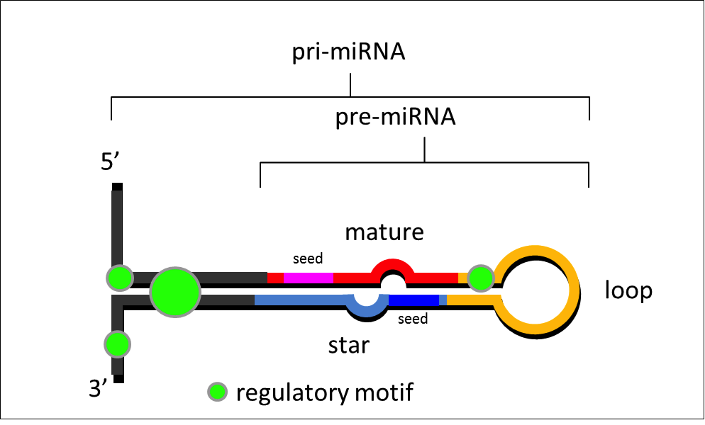
By manually curating all 1'881 putative miRNA entries currently deposited for human in the online repository miRBase (v21) [1], a subset of 521 manually curated miRNA genes that fulfill structural criteria for the annotation of miRNA genes was derived (MirGeneDB.org) [2]. Here, we use this refined human miRNA complement that is annotated in all parts (primary miRNA, precursor-miRNA, mature miRNA including seed, loop sequence, star sequence including seed and its flanking regions (30nts) on both ends), with tracks for each miRNA part constituting a miRNA suite.
Figure 1: Illustration of the different parts of a miRNA
[1] Kozomara, A., and S. Griffiths-Jones, miRBase: annotating high confidence microRNAs using deep sequencing data. Nucleic Acids Res 42(1):D68-73, 2014.
[2] Fromm, B., et al., A Uniform System for the Annotation of Vertebrate microRNA Genes and the Evolution of the Human microRNAome. Annu Rev Genet 49:213-42., 2015.
Analysis using GSuite Tools
Using GSuite Tools we examined whether the genomic regions of the different microRNA parts, as well as whole miRNAs, overlap with commonly occurring SNPs (from UCSC) and SNPs that are associated with different traits (from GWAS catalogue). We compiled the data sets described above and analyzed:
1. The intersection between each GWAS extended SNP dataset (GSuite) against each data set of a particular miRNA part or whole miRNA (GSuite). Annotated analysis history is available on a separate page: Disease-associated SNPs in miRNAs
2. The intersection between the common SNP dataset (track) against each dataset of a particular miRNA part or whole miRNA (GSuite). Annotated analysis history is available on a separate page: Common SNPs in miRNAs
- Results:
- Common SNPs
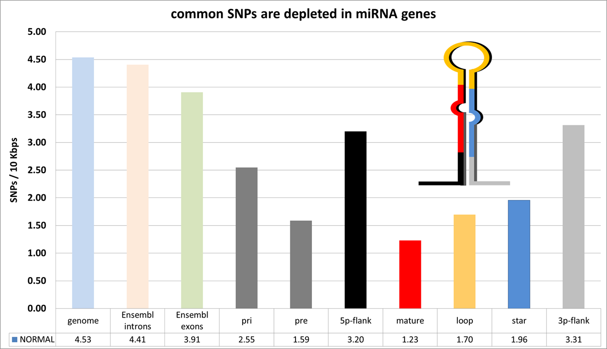
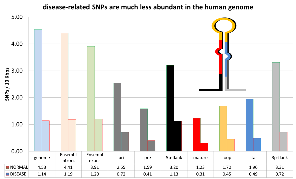
Of the 12'969'631 common SNPs for human, 217 SNPs were observed in 166 of the 521 miRNAs. This corresponds to a SNP density of 2,6 SNPs/10 KB within pri-miRNA. When compared to other parts of the human genome such as the full genome (4,6 SNPs/10 KB), introns (4,4 SNPs / 10 KB) and exons (3,9 SNPs / 10KB) this value is significantly lower underlining the strong selective pressure against changes of miRNAs in general. More specifically we observe a gradual depletion of SNPs for parts of the miRNA precursor depending on their importance for miRNA function (figure 1).
Figure 1: distribution of common SNPs across different parts of the human genome. MiRNA loci show significantly lower SNPs/10 Kbps than the rest of the genome.
- Disease related SNPs
Of these 50 miRNAs, 10 were co-matures, 19 5' matures and 21 were 3' matures respectively.
The SNPs were distributed in all parts of miRNAs but showed the highest prevalence in the 5' and 3' flanking regions of the miRNAs (30 and 19 reported SNPs respectively); possibly within regulatory motifs (UG; CNNC). In line with the observation from the common SNPs the star-sequences showed the next-highest prevalence (5) followed by identical numbers (4) for loop and matures.
Figure 2: distribution of common and disease-related SNPs across different parts of the human genome.
- Relative SNP density
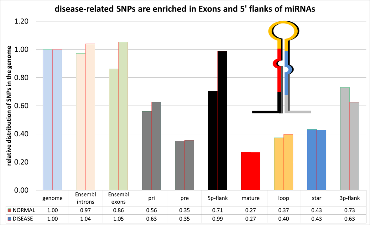
That the total number of disease related SNPs is significantly smaller than common SNPs is known. It was however interesting to see that the abundance of SNPs between the different parts of the genome seemed so similar. A more detailed comparison of the relative density of SNPs (normalized for the ratio of total SNPs to the respective genomic parts in the common SNP dataset) in the disease-related SNPs shows an enrichment of SNPs in exons and 5' flanking regions of miRNAs.
Figure 3: Normalized distribution of common and disease-related SNPs across different parts of the human genome show deviations.
- Chromatin accessibility and mutational profiles of tumors
- Background
Tumor genomes are highly heterogeneous with respect to their mutational burden. This heterogeneity can arise from multiple sources. A common source is exposure to mutagens, such as ultraviolet radiation in malignant melanoma and tobacco in lung cancer [1]. In addition, it has recently been shown that the epigenomic profile (chromatin accessibility, histone modifications etc.) of a tumor's cell-of-origin is highly associated with its somatic mutational landscape [2]. Importantly, such findings may ultimately allow for accurate prediction of cell-of-origin of a cancer based on the somatic mutation profile. In this example usage of GSuite, we will investigate the strong statistical association that was found for chromatin accessibility in melanocytes and the somatic mutation density in malignant melanoma [2] (see wym-1462355009093 ). We will demonstrate through a fully reproducible workflow how this question may be approached within the GSuite framework.
[1] Lawrence M. et al. Mutational heterogeneity in cancer and the search for new cancer-associated genes. Nature 499, 214-218 (2013)
[2] Polak, P. et al. Cell-of-origin chromatin organization shapes the mutational landscape of cancer. Nature 518, 360-364 (2015).
- Datasets used in the analysis:
In order to address the question we utilised the following datasets:
- Whole-genome somatic mutational profiles in melanoma (simple somatic mutations, ICGC)
* SKCA-BR (Skin adenocarcinoma, Brasil)
* MELA-AU (Skin cancer, Australia)
- Chromatin accessibility tracks across cell types (DnaseSeq from ENCODE)
* A549, HepG2, MCF-7, Adult_CD4+, Caco-2, COLO829, Cerebellum, Fibrobl, H1-hESC, HepG2, Hepatocytes, LNCaP, Medullo, Melano (epidermal melanocytes), Mel-2183 (melanoma cell line), Naive_Bcell, Osteobl, PANC-1, PanIslets, SKMC, T47-D
In order to investigate the reported relationship in an unbiased manner, we included a rich set of cell types/cell lines for the chromatin accessibility data.
- Analysis/comments:
The analysis was roughly divided in three parts:
1) Creation of two mutation datasets, each containing somatic variants in skin cancer donors (from the International Cancer Genome Consortium, ICGC)
2) Creation of a GSuite of chromatin accessibility datasets for a diversity of cell lines/ cell types(from ENCODE)
3) Determine the GSuite tracks in 2) that most strongly coincide with the two mutation datasets in 1), i.e. which cell-type specific chromatin accessibility profile is most strongly correlated to the mutation profile of skin cancer?
Steps 2) and 3) were readily accessible within the main functionality of the GSuite framework. The establishment of somatic datasets from ICGC (step 1)) required some additional Galaxy steps (manipulation/filtering) because the raw data contained duplicate entries (due to variant overlap in different transcript isoforms). With respect to the key step in our workflow (3)), we used the analysis available through Statistical analysis of GSuites - Determine GSuite tracks coinciding with a target track. As the track-to-track similarity measure, we chose the Correlated bin coverage, using 1Mb as our bin size (this to resemble the analysis [1]). Here, the chromatin datasets acted as a GSuite, while the mutation datasets were each represented as GTracks. Using this approach, we obtained a similarity score (Correlated bin coverage?) for each of the cell-specific chromatin accessibility tracks in relation to the mutation datasets. Overall, we found that for both the SKCA-BR and MELA-AU datasets, chromatin accessibility tracks for epidermal melanocytes and the Mel-2183 melanoma cell line were ranked as the most dissimilar ones. This finding supports the strong negative correlation that was reported by Polak et al. In conclusion, this example of the GSuite framework demonstrates how a track-based similarity of chromatin accessibility tracks and cancer mutation datasets can highlight the most likely cell-of-origin of a cancer genome.
[1] Polak, P. et al. Cell-of-origin chromatin organization shapes the mutational landscape of cancer. Nature 518, 360-364 (2015).
- Investigating the co-localisation between transcription factors and histone marks
- Background
Expression of genes is a highly complex process where transcription factors and epigenetic modifications play important roles. Transcription factors are able to alter the epigenetic environment of target genes, however, their binding is also influenced by already existing marks. Hence, by investigating which epigenetic marks transcription factors co-localise with it is possible to obtain preliminary information about their regulatory properties.
- Preface:
In this example we are going to investigate the genomic co-localisation between a subset of transcription factors and epigenetic marks known as histone modifications from the K562 leukemia cell line generated by the ENCODE consortium [1]. The epigenetic mark tri-methylation of histone 3 lysine 4 (H3K4me3) and acetylation of the same histone at lysine 9 and 27 (H3K9ac and H3K27ac) are found to correlate with active transcription while the tri-methylation of lysine 9 and 27 (H3K9me3 and H3K27me3) with repression [2-4]. The workflow outlined can be used to investigate the relationship between additional genomic interacting proteins and features, such as DNA methylation and genomic mutations. The data used in the example are genomic areas enriched for the transcription factor or histone modification in question, known as peaks, generated by the technique Chromatin Immunoprecipitation coupled with next generation sequencing (ChIP-Seq).
[1] ENCODE Project Consortium, Bernstein BE, Birney E, Dunham I, Green ED, Gunter C, et al. (2012) An integrated encyclopedia of DNA elements in the human genome. Nature 489: 57-74
[2] Barski A, Cuddapah S, Cui K, Roh T-Y, Schones DE, Wang Z, et al. (2007) High-resolution profiling of histone methylations in the human genome. Cell 129: 823-837.
[3] Mikkelsen TS, Xu Z, Zhang X, Wang L, Gimble JM, Lander ES, et al. (2010) Comparative epigenomic analysis of murine and human adipogenesis. Cell 143: 156-169.
[4] Barth T and Imhof A (2010) Fast signals and slow marks: the dynamics of histone modifications., 35(11), 618-626.
- Datasets used in the analysis:
Annotated analysis history (including all the utilized data and operations) is available on a separate page . (All results mentioned below refer to elements from this history page.)
Initial two GSuites for the subset of histone modifications and transcription factors, respectively, were created using "Create a GSuite from an integrated catalog of genomic datasets" satisfying the following criteria were selected:
Histones:
Track category: Histone variants and modifications (search by cell/tissue type)
Sub-category: K562 Leukemia cell line
Database: All original tracks
File type: narrowPeak
Datatype: Others
Selected subset of tracks manually
Transcription factors:
Track category: Transcription factor binding sites (search by cell/tissue type)
Sub-category: K562 Leukemia cell line
Database: All original tracks
File type: narrowPeak
Data type: narrowPeak
Selected subset of tracks manually
For downstream analysis the downloaded files were used.
In order to count the number of times each transcription factor overlap with a histone modifications the GSuite containg the peaks for the transcription factors was modified to contain only the middle point of each peak using "Modify primary tracks referred to in a GSuite":
Operation: Expand all points and segments equally
Parameter: typed: "middle"
Change file suffix: "Yes" and changed suffix to "bed"
To investigate how the transcription factors colocalizes with the different histone modifications, the two GSuites were preprocessed for analysis using "Preprocess a GSuite for analysis" and secondly a co-localization analysis were setup using "Determine coinciding track combinations from two GSuites" selecting the following parameters:
Query track: GSuite with transcription factors containing the middle point of each peak.
Reference track: GSuite with Histone modifications
Genome: hg19
Similarity measure: Forbes coefficient: ratio of observed to expected overlap.
- Conclusion:
The colocalization shows that the transcription factors overlaps with various degree with the histone marks associated with active transcription (H3K4me3, H3K9ac and H3K27ac) while only a small fraction is overlapping with the histone marks linked to repression (H3K9me3 and H3K27me3).
- Exploring transcription factor co-occurrence using two alternative measures of similarity
- Background
GATA1 is a zinc-finger type transcription factor (TF) with a key role in regulating gene programs during hematopoiesis, where it induces megakaryocytic and erythroid commitment and simultaneously prevents granulocyte-monocyte and lymphoid development (Kitajima et al. PMID: 16543218, Welch et al. PMID: 15297311; Ferreira et al. PMID: 15684376). GATA1 is sequence-specific DNA-binding protein recognizing the GATA box motif (WGATAR) found in regulatory sites controlling its target genes (Trainor 1996, PMID: 8628290).
Approximately 20,000 sites with GATA1 bound are found in the genome of erythroid cells (Ulirsch JC, et al., PMID: 25521328). A recent study which used high-resolution ChIP-exo to map GATA1 and TAL1 across the mouse genome, identified ∼10,000 GATA1 and ∼15,000 TAL1, of which ∼4,000 locations were bound by both GATA1 and TAL1 (PMID: 26503782). The current understanding is that key complexes are formed by combinatorial occupancy patterns of erythroid TFs leading to the induction of key erythroid genes.
- Datasets used in the analysis:
To perform a similarity measure of GATA1 in K562 cells, we collected 318 ChIP-seq datasets from ENCODE (PMID 22955616) and downloaded to history. We then performed similarity testing of GATA1 ChIP-seq track (Snyder lab, Stanford) against the 317 experimental datasets using the Forbes, Jaccard and tetrachoric correlation similarity measures.
- Analysis datasets - history
Annotated analysis histories (including all the utilized data and operations) are available on separate pages for the analysis leading to ranking of tracks and the quantitative analysis of correlation between similarity measures and track sizes . For both histories, the history elements are annotated with details of the performed analysis and their main interpretation.
- Analysis and conclusions:
We generated two separate rankings of the 317 chip-seq tracks, based on their similarity against the GATA1 track according to the Forbes, Jaccard and tetrachoric correlation similarity measures, respectively. In addition to exploring the biological interpretations of the three different rankings, we performed a quantitative analysis of how similarity values correlated with the size of tracks and how the similarity values changed through subsampling of elements from the tracks.
he three alternative measures (Forbes, Jaccard and tetrachoric correlation) resulted in markedly different rankings of similarity to GATA1. With the Forbes measure, another replicate of GATA1 was ranked first, along with several other potentially interesting TFs at the top, but without expected co-binding TFs like TAL1 being among the most highly ranked TF. The ranking according to the Jaccard measure were clearly influenced by size of tracks, with other replicates for GATA1 not being among the highest ranked TF. At the same time, the expected co-binding TF TAL1 was ranked among the top tracks, along with several tracks for GATA2. The results using tetrachoric correlation appeared superior to that of the other measures - including both the other GATA1 track, several GATA2 tracks and the TF TAL1 at the top of the ranking.
To further explore the influence of track size on the measures, we performed a quantitative analysis of the Forbes and Jaccard similarity values. We selected 291 ChIP-seq tracks that had at least 1000 peaks, and made separate Scatterplots of Forbes, Jaccard and tetrachoric correlation similarity versus track size. The Jaccard similarity values was seen to be strongly correlated with track size. To further determine whether this was directly connected to track size, we randomly subsampled a set of 1000 peaks for each track. The Forbes values were essentially unchanged by this subsampling, while the Jaccard values changed substantially. The tetrachoric correlation was affected to some degree, but much less markedly than the Jaccard values. This shows that the Jaccard measure is very sensitive to the number of elements in tracks, and that care must be taken to ensure that biological interpretations are not dominated by technicalities related to the number of discovered peaks.
Note:

This is a specialized version of The Genomic Hyperbrowser, focusing on new functionality for analyzing collections of genomic track. More information on the general HyperBrowser functionality can be found on the main project site.

Contact information

If you have any questions, requests or comments, please use our discussion forum (available from the Help menu) or send us an email to on.oiu.tisu@stseuqer-resworbrepyh‎. We are happy to respond and welcome collaborative projects that help further develop our system. If you encounter any bugs, please let us know via an email to on.oiu.tisu@sgub-resworbrepyh.

If you register as a user, you will be able to subscribe to the on.oiu.tisu@ofni-resworbrepyh mailing list, which serves for distribution of system-related announcements and administrative messages. A backlog of announcements is available from the Help menu. The Help menu also contains citation information.

Source code and more information

Please refer to our GitHub repository for more information about the project and access to the source code, which includes detailed installation instructions. Also, the project page at the University of Oslo web pages provides more research-centric information.

Licensing and support

This project is being developed by the Norwegian bioinformatics community as an open-source project mainly under the GPL license v3 (see the source code for details), supported by various national and local bodies (logos below). It was initiated as a joint project between the Norwegian Radium Hospital (Oslo University Hospital HF), University of Oslo, and Statistics For Innovation.

The Genomic HyperBrowser is an international deliverable of the Norwegian Elixir node. ELIXIR Norway includes the University of Bergen, University of Oslo, the University of Tromsø, the Norwegian University of Science and Technology in Trondheim, and the Norwegian University of Life Sciences at Ås. The Research Council of Norway supports the Node primarily through its program for research infrastructure. The Genomic HyperBrowser is developed by the Elixir Norway node at the University of Oslo, in collaboration with researchers at University of Oslo (mainly at Biomedical Informatics) and Oslo University Hospital HF (mainly at the Norwegian Radium Hospital).

The Genomic HyperBrowser and GSuite HyperBrowser is Copyright (C) 2008-2017 The Genomic HyperBrowser Core Team.